KorillaClub Algorithms Corner
2D Metaballs
Some people asked me how to do this classic demo effect because they wanted to enter the KorillaClub size coding competition but they didn't know how it is done. So I decided to create this mini-tutorial to explain the algorithm behind the effect.
The effect is actually a visualization of a 2-dimensional scalar field. A scalar field is a discrete field of scalar values, like 1, 2, 0.4, etc. For example a regular C array defined like this:
float foobar[] = {0.1, 0.4, 1.3, 0.25, 1.84};
is a 1D scalar field.
And a 2-dimensional scalar field might look like a 2-dimensional array of values like this:
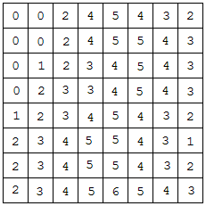
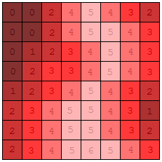
A usual thing to do with a scalar field for metaballs is to classify its points as having higher or lower value than a set threshold, and plot the line (or polygons in 3D) that seperates the two, which requires an algorithm for the extraction of an isocurve (or isosurface in 3D) like marching cubes. However since this is only a 2-dimensional scalar field we can also just directly visualize it by assigning different colors to the values in the field, a common practice being to assign brighter colors to points with higher values. If we visualize the previous scalar field like that we get this result:
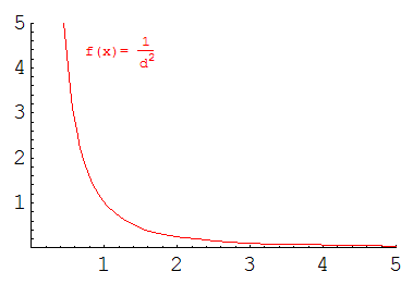
Now the interesting part is how we calculate the values of the scalar field that we are going to visualize. For metaballs the we use an equation from physics, the potential of a point in a magnetic field, which is a function of its distance from the potential source.
Thus the potential of an arbitrary point is calculated by the equation:

And here is the plot of it for illustration purposes.
But there may be a number of potential sources in the field (and there should be or it won't make an interesting effect), so the equation becomes:

where N is the number of potential sources
However the euclidian distance between two points is: 
So the equation becomes:
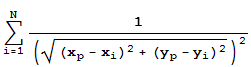
Where, Xi, Yi is the x and y coordinates of the position of source i (where the center of each blob will be), and Xp, Yp is the x and y coordinates of the point (pixel) under consideration (of course this must be done for every pixel).
The square kills the square root so the equation gets simplified to:
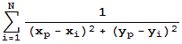
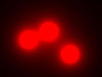
By performing this calculation for every pixel on the screen (considering the screen as a scalar field) and visualizing the resulting field with a gradient palette we get the well known blobs image. Now to animate it we only need to change the positions of the potential sources over time. This is usually done by calculating the position as the result of a sum of sines and cosines of time, just experiment until the motion looks nice.
-- Nuclear / the Lab --